A Science Experiment: part 2
And we’re back! As noted in part 1, there is the possibility I’ve discovered something interesting in biology. Lacking an academic peer group, I’m using a series of blog posts to gather feedback and to keep myself honest. Because chances continue to be high that as an outsider I am deluding myself.
The full backstory can be found in part 1 without which this installment will not make much sense.
Now, to reduce the tension a bit, let me describe the somewhat niche things that I have done, and which I hope could possibly be worthwhile:
- I’ve created & released what I think is the biggest and most comprehensive database of GC/TA & a dozen other skews in 25000 bacterial chromosomes.
- I’ve released and open sourced the software that creates this database after a few hours of crunching on over 120GB of public NCBI data (sequences, annotations, taxonomy).
- I’ve made a simple Jupyter notebook available to explore & plot this database.
- Taking a brief look at this dataset ("SkewDB"), I have found a way to predict GC/TA skew in Firmicute bacteria, and perhaps also explain it, possibly settling some debates.
- With another scan of the database, I have found dozens of bacteria
showing hitherto unexplained behaviour, for which I have found no
useful hypotheses.
- Specifically, many bacteria have asymmetric GC skew, some sporting strands that show no GC skew at all.
- Other bacteria have extremely unevenly sized strands, which is also unexpected.
All of this is only possible because tens of thousands of scientists share their DNA sequences with the world. I for one am very grateful for this openness! Even if none of my small discoveries hold up, I am confident the SkewDB can help other researchers uncover interesting things – assuming I’ve not messed up too badly.
I will write up these things as a more formal preprint, in hopes that actual scientists can review if what I’ve found holds up.
Note - this part of the series is a lot less accessible than part one. I’ve done my very best, but we’re delving into some rather obscure bits of biology. I apologise if I have failed to bring across the sense of wonder – don’t feel bad if this post doesn’t work for you.
Now for the longer story, which covers all the bullet points above:
Getting our hands on DNA
In the previous post I went over a lot of theory, now let’s make it practical. Like most people, I don’t have an actual laboratory to do science with. But the great news is that DNA data is widely shared – if you know where to look.
Let’s start with an infamous bacterium: Clostridioides difficile. A great place to start is the NCBI database, where we can search for Clostridioides difficile. It tells us “Clostridioides difficile is a species of firmicute in the family Peptostreptococcaceae”, and offers options to browse and download genomes. This finds an astounding 12,651 genomes, but if we filter on ‘reference genomes’, we end up with one: GCF_002007885.1. Select this one and press download.
In the resulting ZIP, we find the following files:
Archive:  for-blogpost.zip
Length   Name
-------  ----
   1599  README.md
    373  ncbi_dataset/data/data_summary.tsv
   1119  ncbi_dataset/data/assembly_data_report.jsonl
4176019  ncbi_dataset/data/GCF_002007885.1/GCF_002007885.1_ASM200788v1_genomic.fna
2122958  ncbi_dataset/data/GCF_002007885.1/genomic.gff
    198  ncbi_dataset/data/GCF_002007885.1/sequence_report.jsonl
    598  ncbi_dataset/data/dataset_catalog.json
-------  -------
6302864  7 files
The two large files are the ones we care about - .fna stands for FASTA, and it is the format in which DNA sequences are shared. And it really is quite simple:
>NZ_CP019870.1 Clostridioides difficile strain BR81 chromosome, complete genome
CATAGTATCTTATAATTACTATGATACAGCCTTTTTAATATTATTCAAATTTAAAACAGTTTACATTTCTATTATATTAC
ATATAATTTCAGTAATTTTATATTAATTTTTCTATCTGGAAAAAAATGATTTAAAACTTAAGTTATGATATAATTTCATT
AAAAGAAGGCGATTTTTAGTAAATATGAGAAAATAATGTGTTTTTAGGGGAAAAGTTAAATACAGATTTAAGTGAACAAG
...
TACATATATGGTTAGAAAATGGAGTTGATGTATGTGGATTTGGTGGTTTATTAACTAAAGGTTCTGTTGAAGATATTGCT
AAAAATGCTAAAAAGATTCGTGAAATCATTAAAAATGTAAAAAAAATTTAACATAGGGCTGTAT
And there you have it, actual DNA! You can look at this all day for patterns. This is called ‘sequence gazing’, and it gets you nowhere.
The other large file, ending on .gff, is like a table of contents. It has lines like the following (wrapped a bit for legibility):
NZ_CP019870.1   RefSeq  gene    465     2972    .       +       .
	ID=gene-BZ168_RS00005;Dbxref=GeneID:57296513;
	Name=BZ168_RS00005;gbkey=Gene;gene_biotype=protein_coding;
	locus_tag=BZ168_RS00005;old_locus_tag=BZ168_00005
This says that there is a gene that starts at position 465 and ends at 2972. Inexplicably, they count from 1 in genomics. If we look at that range in the .fna file above, we find:
ATGAAAGAAGACATTGGTTACATCGAATGT ... AAAAGAAGCATACCTATGTACTAGCATGATTTAA
^^^                                                               ^^^
Genes start with a start codon, and this is nearly always ‘ATG’. And indeed, that is what we find here. Genes end on one of three stop codons, TAG, TAA or TGA. And indeed, this gene ends on TAA. So it all works!
Some statistics
When I started as a guest researcher over at TU Delft Bionanoscience, I created open source DNA processing software called Antonie. Antonie creates a lot of statistics for a genome, this is an excerpt:
| name | NZ_CP019870.1 |
|---|---|
| fullname | NZ_CP019870.1 Clostridioides difficile strain BR81 chromosome, complete genome |
| acount | 1468605 |
| ccount | 595727 |
| gcount | 588291 |
| tcount | 1471761 |
| siz | 4124383 |
From this we can see that this chromosome consists of 4124383 nucleotides. In addition, we see that there are very similar numbers of A and T nucleotides (acount/tcount). Also, the G and C numbers are very similar. This is a very common finding.
Funnily enough we don’t quite know why this happens! If you count the letters in DNA, in almost all organisms, you’ll find that “%G ≈ %C” and “%T ≈ %A”. However, there can be way more GC than TA or the other way around. Somehow only GC and TA are in sync among themselves.
I continue to find it strange that such an odd phenomenon at the core of biology is so poorly understood. There are arguments that say this is just chance, that if you flip a coin a million times, it is no great miracle that heads and tails both happen around 500k times. Perhaps this is so, but why does the rule only hold for G/C and A/T? The Wikipedia page in Chargaff’s second parity rule makes for some fascinating reading.
GC skew
As noted in part 1, DNA gets copied in two different ways. In bacteria, one half of the chromosome always gets copied in a straightforward way (leading strand), the other half via a complicated forward/reverse process (lagging strand).
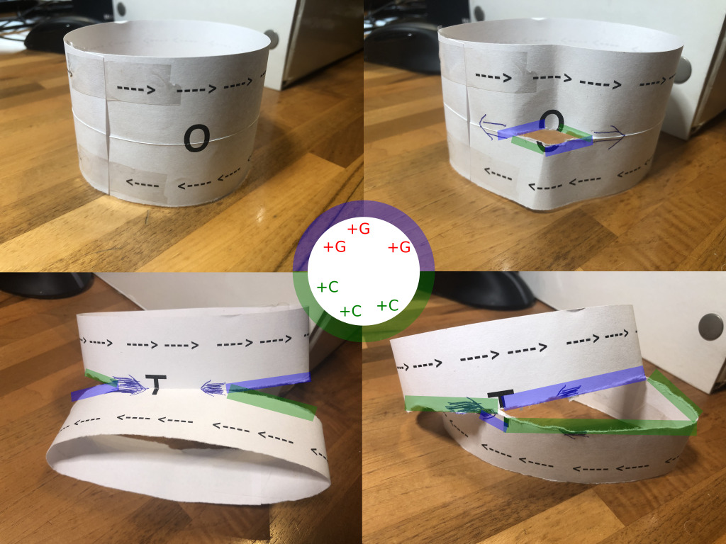
Bacterial chromosome being copied in two directions. Main takeaway is that the blue and greenish halves got copied in opposite directions. In this photo, the blueish part accumulates some extra G’s, and the greenish part some extra C’s
To clarify this a bit, imagine the chromosome as laid out in the photos above, starting at the upper left corner. Note how the top and bottom half of this paper chromosome have arrows pointing in opposite directions. These denote the natural processing direction of the DNA (“3’ -> 5’”).
The “O” denotes the origin of replication. And in this case, much as in real life, the replication process starts by tearing up the chromosome. This is the top right photo. Note that the tear proceeds in opposite directions if we continue to pull the strands apart. One part of the tear moves in the same direction as the top DNA direction (the arrows), the other one in the same direction as the bottom DNA direction. This is very comparable to what happens during real life chromosome replication.
The tearing apart continues until we reach the opposite site of the chromosome, where we find the termination sites (T). And finally, we have two separate chromosomes.
In real life, the chromosome doesn’t just get torn apart, during this process “complementing” happens, which means that we don’t end up with two partial chromosomes, but two whole ones. In a delicious twist, due to topological reasons, actual freshly copied chromosomes are catenated, or in other words, they are like two interlinked chain links, running through each other. A separate enzyme then briefly cuts the chromosomes so they can truly be separated.
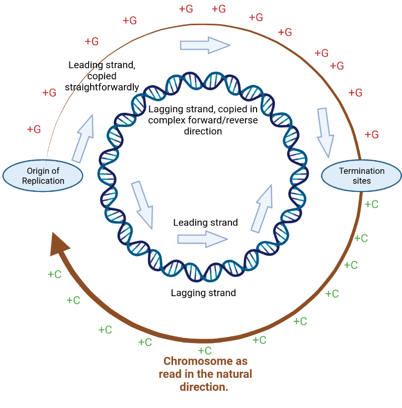
Bacterial chromosome copying - image made with Biorender
In this slightly more factual schematic, the copying processes also starts at the Origin of Replication. One part travels “up” in this picture, on the outside DNA strand. The other one goes downwards, on the inner DNA strand (as drawn). This can be compared to the tear in the paper chromosome above proceeding in opposite directions.
And much like in the paper chromosome, the two “copying forks” run into each other at the termination sites.
The upshot of this is that 50% of each strand is copied in the forward direction (the ’leading strand’), and 50% in the reverse direction (the ’lagging strand’).
(If this concept is unclear at this point, it may help to jump back to part 1 and watch the video again - this stuff is hard to understand)
Over the millennia, the differing copying processes leave traces in the DNA. In almost all bacteria, the leading strand shows an excess of G nucleotides over C nucleotides. The lagging strand then shows the reverse. This is shown in the picture as the little “+G” and “+C” labels.
In general, the amount of G and C nucleotides over the whole genome is almost equal however. Just not everywhere - the strands differ! And why does this happen? We don’t really know. As the Wikipedia notes:
“There is lack of consensus in scientific community with regard to the mechanism underlying the bias in nucleotide composition within each DNA strand. " – Wikipedia entry on GC skew
So what does this look like? One way of plotting this is to use the “cumulative GC skew” (Andrei Grigoriev, 1998). This means we go over an entire genome, and every time we encounter a G, we increase a counter. Every time we see a C, we decrease it. And if we do so for C. difficile, we end up with this:
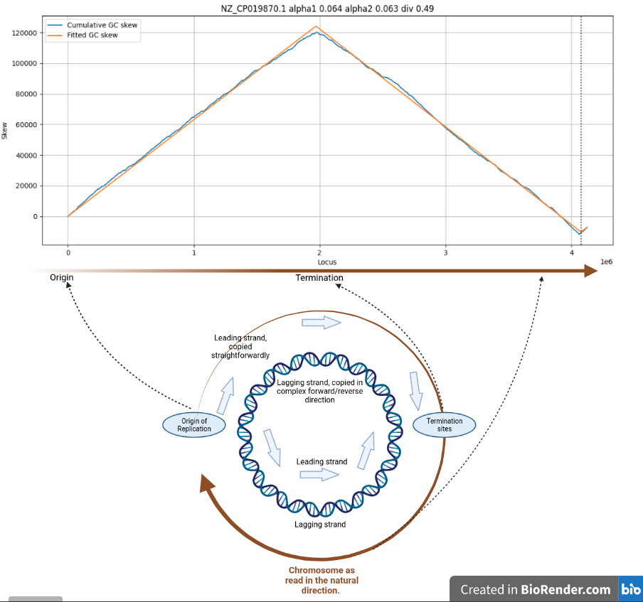
Cumulative GC skew for C. difficile
The x-axis is the position in the chromosome, going from 1 to 4124383. The y-axis represents the cumulative skew, the counter from above.
The blue line is the reality, the orange line is a fit used for further analysis. The blue line goes up, and down, at a rate of “0.064”. This means that for every 1000 nucleotides, the cumulative GC excess changes by 64.
Note the very sharp corners - these are located at the transition between copying in one direction (simple) and copying in the other direction (very complicated).
Unlike computer files on disk, bacterial chromosomes are circular and have no physically defined beginning or end. It is however customary to start the .fna file with the DNA sequence more or less at the Origin of Replication, where the DNA copying process starts.
Here we see that the creators of the reference genome (Kyung Hee University) for C. difficile got pretty close - the actual beginning is off by around 100k nucleotides. This is of no practical significance, although “strange GC skew” can be used to detect DNA sequencing problems.
Bulk analysis
Using the Antonie software, it is possible to analyse the roughly 25000 chromosomes for which we have data. This forms the SkewDB. For all chromosomes this contains:
- GC & TA skew (also per codon position) graphs & parameters
- Strand bias (the extent to which genes prefer one strand)
- Codon bias (more about which later)
- Percentage of non-coding nucleotides
- Taxonomic data (bacterial family etc)
This is all deposited in a bunch of CSV files, which can be joined together into one big one, which I have uploaded here. In addition, for every chromosome, this delivers a separate CSV file that plots how well fit and reality agree. I’ve bundled these CSVs here.
And, to get you started here is a Jupyter notebook that creates most of the graphs on this page, based on these two files.
As far as I know, creating such a large public database has not been done before. Jean R Lobry discovered GC skew in three genomes way back in the mists of time of 1996, when this would have been very hard work.
The DoriC database (Hao Luo, Feng Gao* (2018)) documents details of the Origin of replication in genomes (oriC), and also has a database of skews (the “Z-curve”).
Then there is the SkewIT index as calculated by Jennifer Lu and Steven L. Salzberg, but this is a single number. They provide a helpful web app for calculations here.
In contrast, my data set shows separate details for 10 kinds of skews, including parameters per strand - which enables us to discover asymmetries, for example.
Some examples
As noted, it is not understood well why G and C are usually balanced so closely. In addition, it is not very clear why this is only true for whole bacterial chromosomes, while one half has an excess of G and another one an excess of C.
If we ever want to find this out, we could do a lot worse than to look for patterns among tens of thousands of bacteria, to see if anything jumps out.
With this data set, this is real easy.
One hypothesis is that the GC skew effect is caused by strand bias.
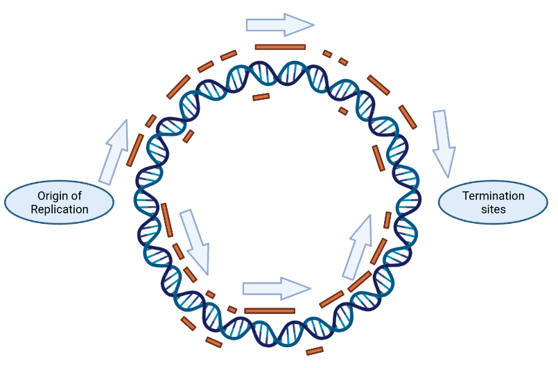
Bacterial chromosome showing replication directions & gene locations (in orange). Made using the pretty awesome Biorender website
Genes can live on both sides of the double DNA helix. It turns out that they tend to huddle on the strand that gets copied straightforwardly (the “leading strand”), as shown in the graphic above. This is called strand bias.
In addition, genes are known to contain more G nucleotides than C nucleotides. This is caused by the codon bias. This means that the whole GC skew phenomenon might be caused purely by the combination of strand bias and codon bias. Because if there are more genes in one half, and these genes contain more G, that would cause exactly the observed skew. Let’s try out this theory with the Antonie dataset:
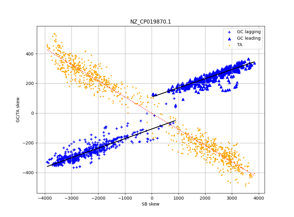
Scatter plot local skew levels (y axis) for C. difficile, and the local gene strand bias
In this scatter plot, I use the Antonie SkewDB data for around 1000 overlapping pieces of the C. difficile genome, and for each of those pieces plot both the strand bias (“how many gene positions are on this side of the helix”) and the GC and TA skew for that piece. And something interesting jumps out immediately.
First we can look at the TA skew (which is the same idea as GC skew, but now for T and A). These are the orange dots and the orange line - this is a pretty good fit! And, it goes straight through the origin of the graph. In other words, on average, pieces with no strand bias also have very little TA skew.
For GC skew something similar is going on, but it turns out the best fit is made when we draw separate lines for the leading (straightforward) and the lagging (complicated) strands of the chromosome. These are the blue markers and lines.
We still see that more strand bias leads to more GC skew - but we also see that it never goes to zero! There is an additional offset that is independent of strand bias, but does depend on which strand we are on.
We can therefore conclude that within C. difficile, TA skew is driven purely by strand bias, but that for GC skew an additional independent strand effect is going on.
More results from SkewDB
C. difficile is one of the most famous members of the Firmicutes phylum of bacteria. We can wonder, does the effect we found hold for the other Firmicutes as well?
To make one big graph, we have to include some more data - like for example how strong the codon bias is for each bacterium. Because the stronger the codon bias, the stronger impact of the strand bias. We also have to adjust for parts of the genome that do not carry genes on either strand.
When we do this, the following graph comes out, where each dot represents one of around 4600 bacteria:
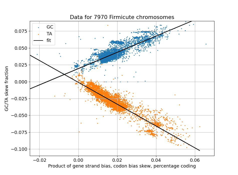
Scatter plot of observed GC skew levels (y axis) and a calculated predictor (x axis)
And this confirms what we saw for C. difficile - if there is no strand or codon bias, there is also no TA skew. And the rule for GC skew generalises as well - even in the absence of these biases, some GC skew remains.
I am not the first one to look at GC skew in Firmicutes of course:
- Atypical at skew in Firmicute genomes results from selection and not from mutation
- Inferring Adaptive Codon Preference to Understand Sources of Selection Shaping Codon Usage Bias
- I maintain a list of other interesting papers here
Some other interesting things
- Many chromosomes show asymmetric GC skew. In some cases, one strand has
no skew at all. The current hypotheses I see for GC skew do not cover
this scenario
- Notable examples: NZ_CP018228.1, NZ_CP072162.1, NZ_CP071399.1, NZ_CP035713.1.
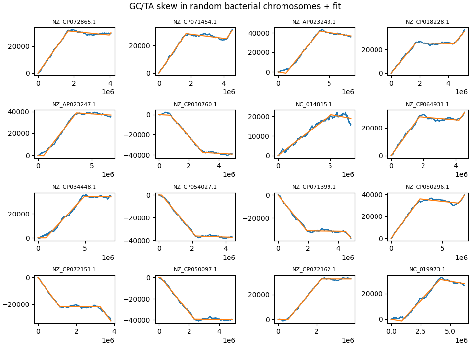
Some random chromosomes where one strand shows no GC skew
- It appears some chromosomes have a very big discrepancy in lengths between the
leading and lagging copying strands. Or in other words, the termination
site is not centered. This should be pretty bad for a bacterium, so it
might be well worth investigating what is going on.
- Notable examples: NZ_CP016636.1, NC_006512.1, NC_018866.1, NZ_CP058983.1.

Some random chromosomes where the leading/lagging strand length disparity is very large
Finally
In the next and probably final part, I’ll explain exactly how to get the software going and what all the fields in the various CSV files mean.
Meanwhile, I hope that some researchers may already be able to benefit from:
- The Antonie SkewDB as CSV
- The 25000 files showing the fit per chromosome
- and the simple Jupyter notebook that shows most of the graphs from this page
If the above is of any use to you, or if you have any questions, please email bert@hubertnet.nl, or try @bert_hu_bert on Twitter.
I’ve also added a comment section, and I’d love to see your questions or remarks here as well: