A Spherical Cow Model of Global Warming (With Data and Code)
Before we start, I’d like to thank ESA’s Mark McCaughrean who helped kick off this article by referring me to two key articles that lay out, in scientific terms, how global warming really works.
Here you can pick your favorite temperature unit: C F (Test temperature: )
Feel free to skip this wordy intro and head straight to the model, or even to the summary at the end of this post!
I must also acknowledge this thread by Markus Deserno which opened my eyes in 2022 that global warming is more complicated than almost everyone thinks. And it turns out it is even more complicated than can fit in a thread.
This work is in some sense data & code driven tribute act to dr Sabine Hossenfelder’s 20 minute video “I Misunderstood the Greenhouse Effect. Here’s How It Works”. And like Sabine’s video, much of what you’ll read below hails from the grand book “Principles of Planetary Climate” by Raymond T. Pierrehumbert. Sadly not all Hossenfelders materials are as good or factual. At the very end this page you’ll find a large list of other sources that I found useful.
Finally a warm thank you to the handful of climate scientists and (atmospheric) physicists that supplied suggestions and clarifications, and also provided some comfort that my story here really reflects the mainstream understanding of the atmospheric physics of global warming.
If you just want a tl;dr of how global warming works, there’s a quite complete summary at the end of this article.
CO₂ & Global Warming
CO₂ is good at trapping heat, and it has a leading role in global warming. However, some people don’t like this fact, and periodically it is rediscovered that CO₂ and water vapor are so good at trapping infrared radiation that the lower atmosphere already captures almost all of it, and that adding yet more CO₂ would therefore not be very harmful, because global warming is already “saturated”. This is not true, and already in 1896, Svante Arrhenius had figured out how things really worked.
And even earlier, Eunice Newton Foote had measured that CO₂ absorbed heat from sunlight, and she theorized this might influence the Earth’s temperature.
It turns out that CO₂ and global warming are superficially simple (“CO₂ traps heat”), but as soon as you study it in any depth it all becomes fiendishly complex. And this complexity leaves ample room for people to sow doubt. Sadly, the complexity also makes it a challenge to satisfy reasonable folks who just want to know what is going on. You just can’t summarise the CO₂ situation in a few sentences.
Instead, this page will use more words than that to give you a solid handle on how our atmosphere traps & releases heat.
Recently dr Sabine Hossenfelder released a 20 minute video that explains it all very well, and her work was viewed 750k times, which is encouraging. This follows efforts in the 1900s, 1950s, 1960s, 2000s and 2010s to also rebut the “CO₂ is already saturated theory”.
Yes, I do know that Hossenfelder has also published questionable stuff. But this video is useful.
This page reads well together with the Hossenfelder video, but you could also decide to only read this page, it is a standalone effort. Whereas the video is very visual, this page has more code (Jupyter playbook in this separate post), more math and more numbers. But both show the same information, just in a different way. For best understanding, I’d recommend watching both the video & reading this page, since this will illuminate a difficult subject in overlapping and complementing ways.
In what follows we’ll be building up a “spherical cow” model of the atmosphere. A spherical cow model attempts to simplify things sufficiently so that we can feel we understand the problem, while retaining enough reality that the resulting numbers are also physically relevant. Specifically, the model is good enough that it can very effectively rebut the “CO₂ is already saturated” theory.
More background is available in a companion blog post that spends more time on physics, math and code (partially in FORTRAN no less!). You might also want to read my earlier post on climate change and management as background.
Very important to note is that our “spherical cow”-grade model is of course not correct (no model is), but it strives to be educational and capture the key effects.

Spherical cows are easier to model, but lack crucial detail compared to real cows. Animation via Wikipedia contributor Keenan Crane
I’m VERY interested in hearing about mistakes in the calculations that follow, but there is no need to tell me the model is a huge simplification. There is also really no need to send me alternative research that somehow refutes the reality of global warming! I’ve included a checklist in the companion post that can help determine if research is serious. Also, do please email me on bert@hubertnet.nl with questions and corrections, though.
This post has been studied by a few professional climate scientists (thanks!), and the feedback is mostly that there is more to climate change than just the atmosphere. But I have received no negative feedback or reports of any (glaring) factual errors. I do remain interested in hearing about problems of course!
Starting the model
To a very good approximation, the Earth only receives energy via sunlight, and only loses it by Outgoing Longwave Radiation. This is one of the very few simple things in climate modeling, and we are going to take immediate advantage of this fact.
The incoming power density from the sun is called the solar constant (\(G_{SC}\)), and it is \(1362W/m^2\), plus or minus 0.2%.

Earth, receiving sunlight and emitting outgoing longwave radiation (OLR)
If we denote the Earth’s radius by \(R\), this means the incoming amount of power is \(\pi{}R^2\cdot{}G_{SC}\), the area of sunlight that the Earth intercepts, multiplied by the solar power density.
Furthermore, if we model the Earth as a completely black sphere with no atmosphere, according to the Stefan–Boltzmann law it will radiate \(4\pi{}R^2\cdot\sigma{}T^4\) of power back into space (the whole surface area times the black body radiation density. \(\sigma\) is the Stefan-Boltzmann constant).
To figure out what temperature this Earth would be, we can calculate at which temperature incoming and outgoing power are equal:
\[ \begin{aligned} \pi{}R^2\cdot{}G_{SC} &= 4\pi{}R^2\cdot{}\sigma{}T^4 \\ G_{SC} &= 4\sigma{}T^4 \\ T &= \sqrt[4]{\frac{G_{SC}}{4\sigma}} \\ T &= 278.4K \end{aligned} \]This corresponds to around . The actual average temperature of the Earth is roughly , so not the worst match. We might be feeling rather good about our simple calculation right now. Let’s make it a bit more accurate, and ruin our mood.
The actual Earth is not a black body, and close to 30% of the incoming solar radiation is reflected straight back into space by things like land, clouds, ice sheets and aerosols (soot, dust, other floating particles):

Earth, receiving sunlight, reflecting a part, and emitting outgoing longwave radiation (OLR)
If we call the reflected fraction \(\alpha_{sb}\) (also known as the albedo) this then leads to:
\[ \begin{aligned} (1-\alpha_{sb})G_{SC} &= 4\sigma{}T^4 \\ T &= \sqrt[4]{\frac{(1-\alpha_{sb})G_{SC}}{4\sigma}} \\ T &= 254.6K \end{aligned} \]This is a rather frigid , very far away from the truth. Although this model does not describe our current environment at ground level, it does contain an important truth: if the Earth is to use black body radiation (the outgoing longwave radiation, OLR) to radiate out all the energy it receives from the sun, it will have to do so at a temperature of . Just not necessarily at ground level. This will turn out to be key later on.
The atmospheric blanket
In reality, the average surface temperature of the Earth is around . Some climate skeptics claim that global warming is already “saturated”, and that further greenhouse gases will not add more insulation. Let’s believe them for a minute and see what would happen:

A thin atmosphere that totally absorbs infrared radiation
Here for ease of drawing we’ve moved to a flat presentation, but if you will, imagine the gray atmosphere as a band around the circular Earth from the earlier diagram above.
This idea was gratefully borrowed from the “Sixty Symbols” video The Greenhouse Effect Explained
Down from the sun comes 70% of the solar constant power (100% minus the 30% that was reflected back into space). Spread over the whole surface (including night time) this is \( (1-\alpha_{sb})\cdot{}G_{sc}/4=238.35W/m^2\) . All of this makes it to the Earth’s surface (in this diagram, at least. In reality, the atmosphere does absorb a small part of the incoming solar radiation).
Again, no energy leaves the Earth except through radiation. Since this model atmosphere is entirely opaque for outgoing infrared radiation, it must do all the radiating back into space itself. No infrared from the Earth makes it (directly) past the atmosphere here.
This means this atmosphere must radiate back that same 238.35W into space, otherwise the whole Earth would heat up, and we are looking for the stable temperature.
Black body radiation comes from the surface of an object, which in this case also includes the lower end of our opaque atmosphere, which will radiate \(238.35W/m^2\) downwards.
Because the atmosphere has two sides to radiate from, both radiating \(238.35W/m^2\), it needs \(2\cdot{}238.35W/m^2 = 476.70W/m^2\) from the Earth’s surface to maintain a stable temperature.
Like above, the Earth’s infrared radiation is given by \(\sigma{}T_s^4\). If we set that equal to \(476.70W/m^2\), we get Ts=. Balmy! And clearly incorrect. Apparently the real atmosphere is not thin and entirely opaque/saturated.
Now, this is a very simplistic model, specifically because it models a thin atmosphere that has the same temperature at the top and the bottom.
Crucially, in this incorrect model, the entire atmosphere is at the temperature we calculated earlier, the temperature at which the upwards black body radiation is equal to the incoming 238.35W/m2 (from the sun).
But what about Venus?
The nice thing about climate models is that we can test them not just on Earth, but also check how they’d work on other planets. The king of the greenhouse gas effect is of course Venus. Despite being closer to the sun, Venus absorbs less energy from the sunlight than we do: 163W/m2. This is because Venus is so much brighter than the Earth, which on a good day you can see for yourself: Venus can be so bright in our sky that it gives you a shadow on Earth. Venus reflects around 70% of the incoming sunlight.
Yet, its surface temperature is 737K (!). Now, the atmosphere of Venus consists almost entirely of CO₂. Or in other words, compared to the Earth’s 420 ppm (parts per million) of CO₂, Venus has a full 965,000 ppm of it (!). But previously we saw that Earth even with a completely saturated (but thin) atmosphere would only be 303K (29.65C). So what gives?

The thick atmosphere of Venus that totally absorbs infrared radiation
From this it is clear that Venus has a massive atmosphere. Where on Earth most of the atmosphere is gone 20 kilometers up, the Venusian atmosphere is still appreciable at 50 kilometers. Given the incoming solar radiation of 163W/m2, using \(\sigma{}T_s^4\), we can calculate that the \(T_{toa}\) top of atmosphere temperature must be 231K. That’s a far cry from 737K at the surface.
If you stand on top of a mountain, it is a lot colder there than on the ground. In our atmosphere, the temperature drops by around 6 degrees per kilometer going up. This is called the ‘lapse rate’, and at a basic level the cause is some really simple physics (although it quickly gets complicated). Molecules higher up in the air have more potential energy (because of gravity), and thus less kinetic energy (as long as the molecules mix). And this kinetic energy is what we call temperature. This is just like how a waterfall is (slightly) hotter at the bottom than at the top.
The “dry” lapse rate in a dry atmosphere is a very simple function of the gravity divided by the heat capacity of the atmosphere. On Venus, this comes down to 10K/kilometer. We know the (effective) top of the Venusian atmosphere is around 231K. We also know that the temperature will increase by 10K/kilometer as we go down the 50 kilometers of the atmosphere - leading to a guesstimate of the surface temperature of 731K (231K + 10K/km * 50km), which is unreasonably close to the actual temperature of 737K.
This accuracy is mostly a coincidence - there are many complicating factors we did not include in the calculation. But, that the outcome is in the right ballpark should give us some confidence in the method. The spherical cow is producing reasonable predictions.
One other thing to note is that in the Venus calculation, we assumed that the bottom of the atmosphere has the same temperature as the surface. We did not do this for the Earth calculation. The reason is that the extremely dense Venus atmosphere, which is nearly liquid at the bottom, has a 50 times more intense heat exchange with the surface than the Earth has, which makes the Venusian atmosphere and surface have nearly the same temperature.
Radiative transfer on Earth
Because the Venusian atmosphere is a wall of nearly pure CO₂, the calculations there are relatively easy. The Earth’s atmosphere is massively more complicated, mostly because it contains copious amounts of water at lower attitudes, but not at higher elevations. And water is a stupendously complex molecule.
Let’s start with the good news. The surface of the Earth radiates like a near perfect black body. Here is the black body spectrum for the surface of the Earth and that of sunlight:

Earth surface radiation and incoming solar radiation
From this graph we can learn a few things. For one, incoming sunlight and outgoing infrared radiation barely overlap. Secondly, we learn that atmospheric scientists like to use “wavenumbers” in units of \(cm^{-1}\) instead of wave length or frequency in Hz. This has a number of advantages, but it takes some getting used to. We’re operating in their field now, so we’ll have to adjust.
One advantage is that the area under radiation graphs in wavenumbers is representative of the total emitted power, which is visually helpful.
The surface and the lower atmosphere
The lower part of the atmosphere has four relevant greenhouse gases: H₂O (water), CO₂, CH4 (methane) and N2O. In general, atmospheric molecules with only 2 atoms (like oxygen and nitrogen) generally do not interact with infrared radiation (except sometimes).
CO₂ concentration is around 420 ppm these days. In tropical climates water vapor can easily reach 40,000 ppm. Even outside the tropics, 10,000 ppm (1%) is common. That’s a lot.
We know the earth surface radiates infrared radiation upwards, and we’d like to know what the real atmosphere does with that: which parts of the spectrum will be absorbed? And which part gets to go to space? Let’s start with water, since there’s so much of it.
If we search online for “the absorption spectrum” of water… we won’t find it. Because it turns out this spectrum depends on temperature, the square of the water concentration itself (!), presence of other gases and the total pressure. That’s a lot of variables. Anyone that shows you “the” spectrum of water is hoodwinking you. Here’s what it looks like in practice for lower atmosphere temperature, pressure and concentration:

More background on absorption, databases and units used can be found in this companion blog post.
Pretty messy. If we zoom in, we see why there isn’t a simple “water absorption table” you can download - the peaks move left, right, up and down based on all factors mentioned above:
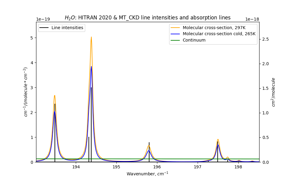
Note how the blue and orange peaks are not quite centered on the black lines
The blue and orange peaks correspond to “rotational-vibrational modes” of the water molecule, and we have a good understanding of how these work. Their origin is in the black vertical lines, which represent the intensities of discrete energy transitions.
In addition to these peaks there is a “continuum spectrum”, shown here as the lower green line. And here’s the thing. We don’t really know where that spectrum comes from. There are various theories which can’t all be true. We do know the continuum spectrum scales with the square of the water pressure (!). And also, that its intensity scales with varying but high powers of any temperature increase. Yes. In addition, over the past 30 years, our measurements of the strength of the continuum spectrum (at higher frequencies) have somehow changed by over an order of magnitude. As of 2023, the data still hasn’t quite settled, specifically for shorter wavelengths, but we’re getting a handle on it.
Although per wavenumber the continuum spectrum is weak, it is present over a very large frequency range which means that integrated it has a major effect on global warming. Which makes it all the more terrible that we don’t really understand it nor spend enough effort on measuring the continuum spectrum.
It is apparently so embarrassing that we don’t understand the water continuum spectrum that it isn’t even mentioned on the Wikipedia “Electromagnetic absorption by water” page!
So, what do these numbers mean in a real atmosphere?
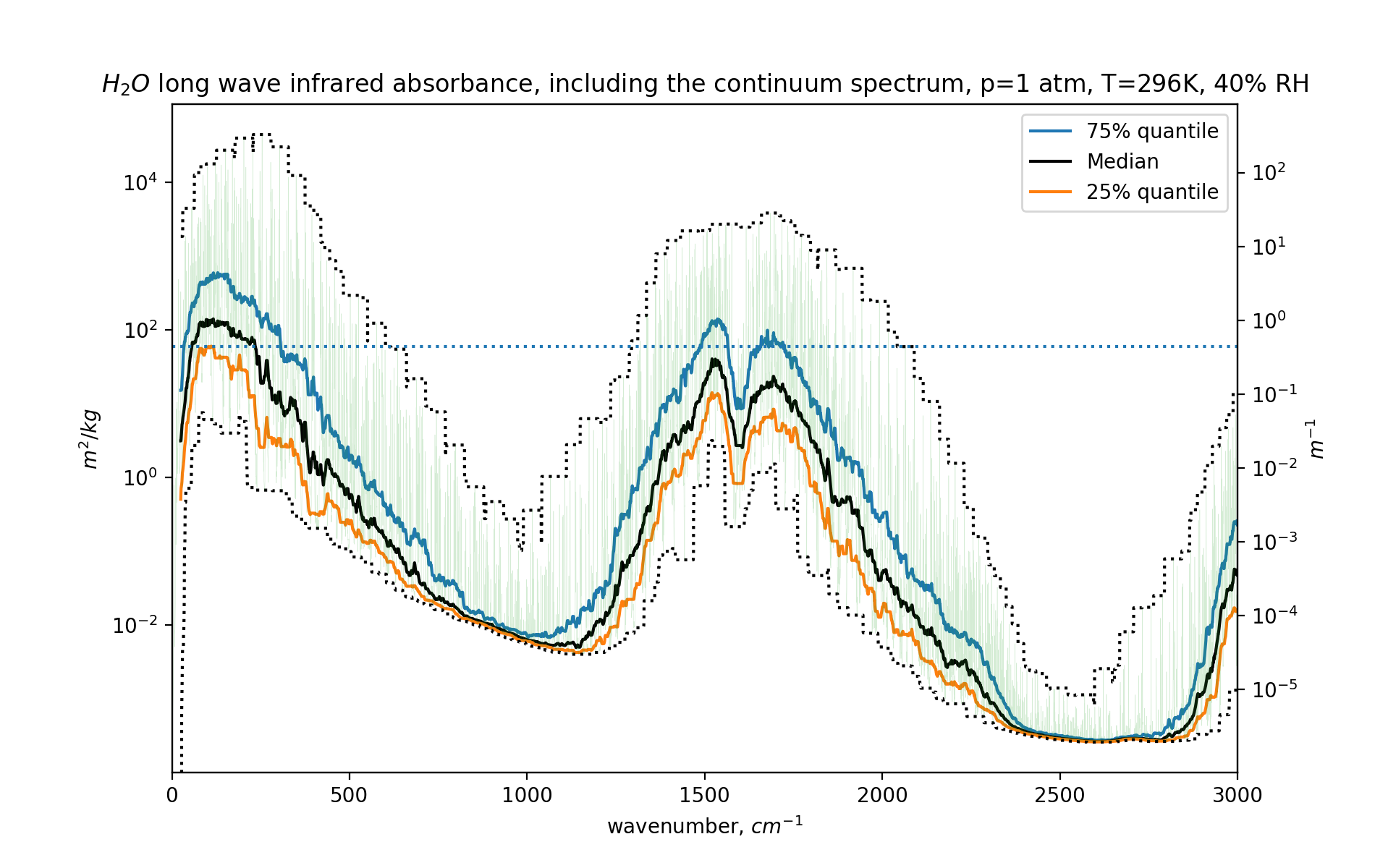
Here we see the attenuation caused by water under realistic surface air conditions - room temperature, 40% relative humidity, normal atmospheric pressure. The black central line is the median of water’s behaviour over a width of 50 wavenumbers. The green chaotic lines are the actual unsummarised characteristics.
On the x-axis are wavenumbers corresponding to outgoing long wave radiation from the Earth’s surface.
On the right y-axis we see a ‘per meter’ number. This is the linear attenuation coefficient for our atmosphere (including the water vapor). If that coefficient is 1, that means the intensity of light decreases by 63% per meter (a factor of \(1/e\)). If the linear attenuation \(\mu\) is 0.1, the intensity will decrease by 63% every ten meters. Or in other words, if \(I\) is the intensity of light, \(I/I_0 = e^{-\mu\cdot{}\textrm{distance}}\). On the left side we see the attenuation per kilo per square meter (more about this in the companion blog post).
From the graph we see that this attenuation is bigger than 0.001/meter for many frequencies, meaning that (say) 5000 meters of air reduces the intensity of light at that wavenumber to near zero. Or in other words, for large parts of the outgoing radiation spectrum, water vapor causes the atmosphere to be opaque. Almost nothing “gets out” at those frequencies, because of water.
Here is what that looks like for the lower 500 meters of our chosen atmosphere:
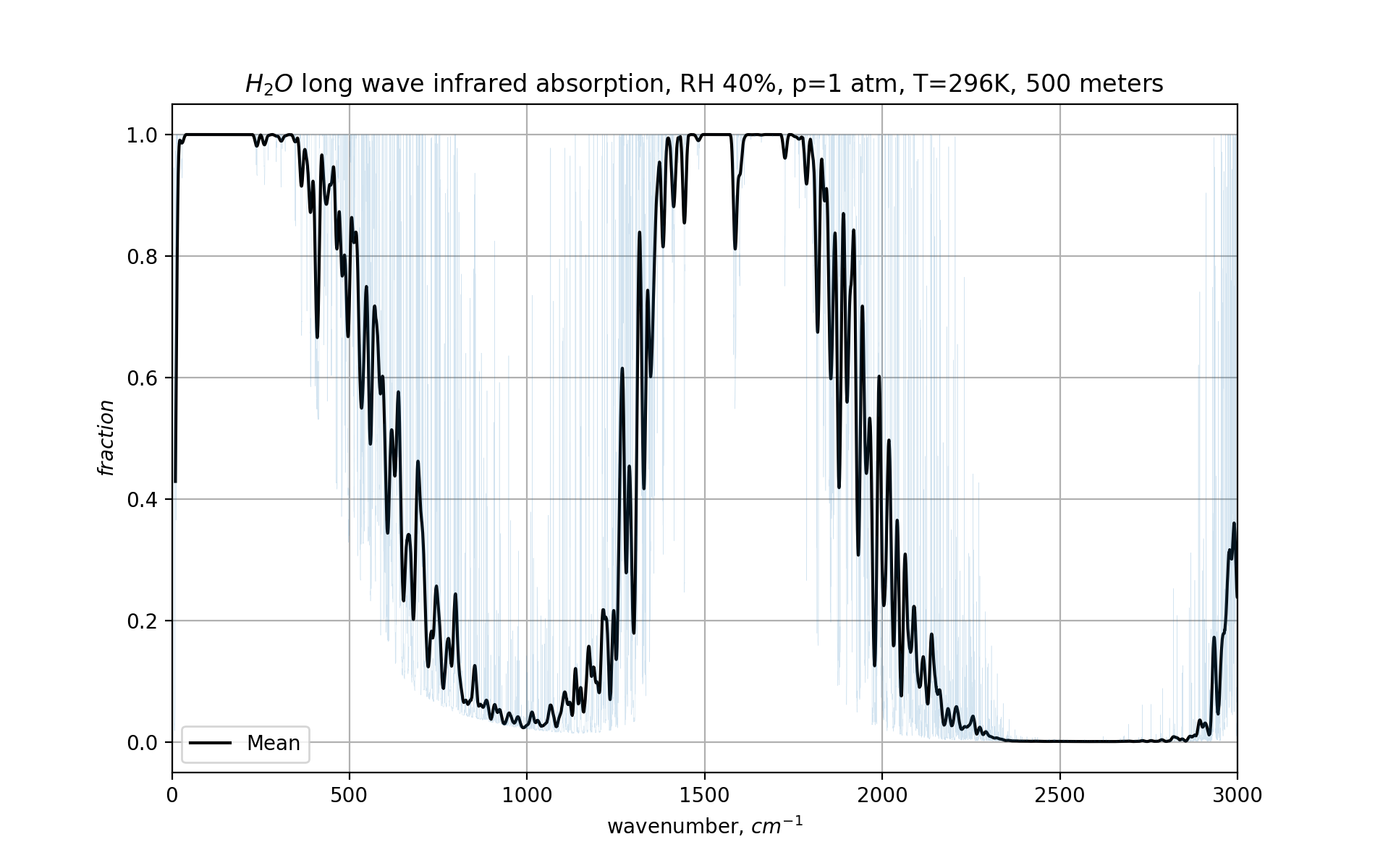
This plots how much light gets absorbed. Below 350 cm-1, nothing gets out. Similarly, between 1500 and 1700 cm-1, almost nothing escapes even these first 500 meters of atmosphere.
Now let’s add CO₂ to the mix:
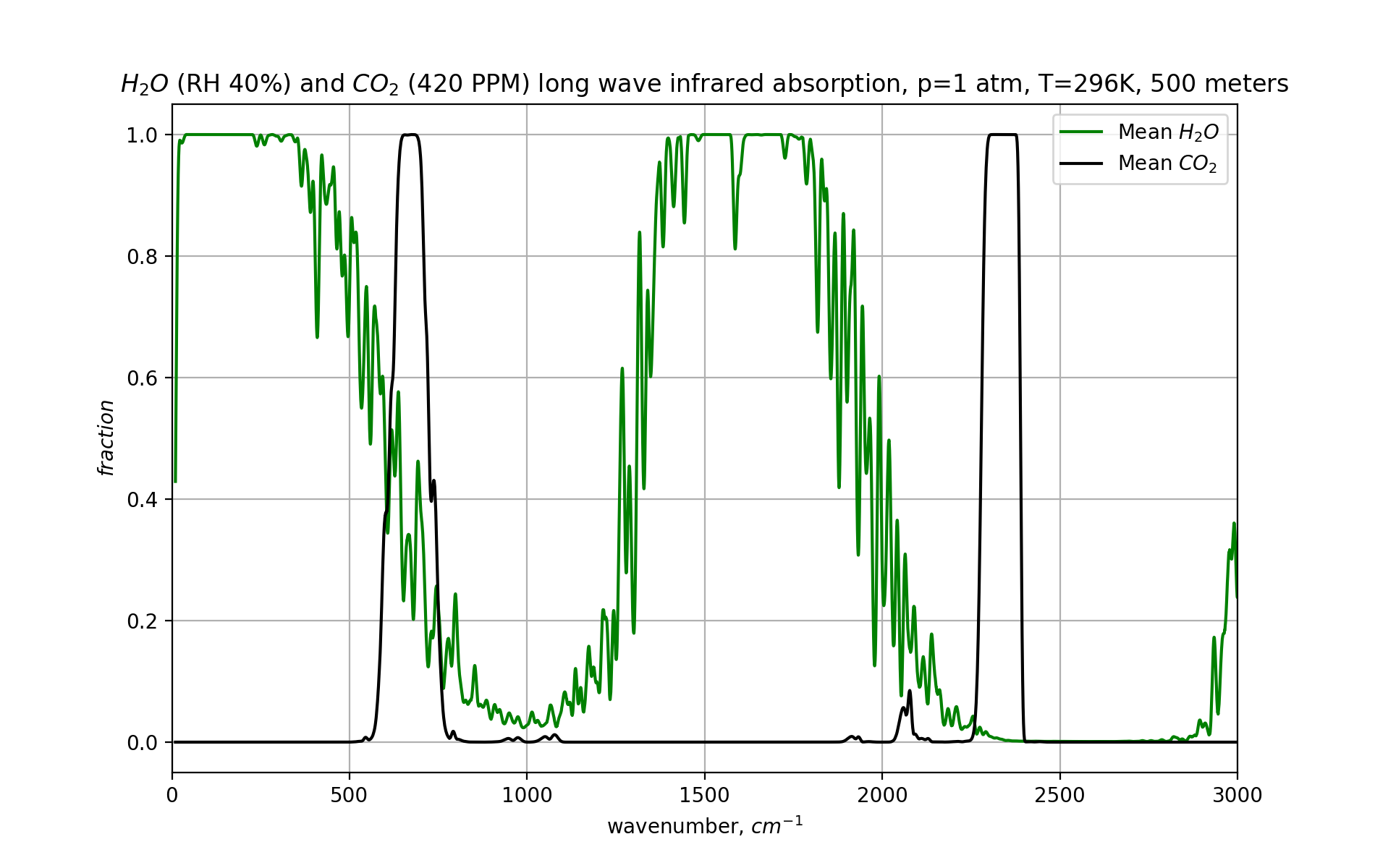
Here we see the oft repeated point that water is a bigger greenhouse gas than CO₂, which is true in the lower atmosphere. A photon with a wavenumber of 650 cm-1 would most likely be absorbed by CO₂, but at that same frequency, water is also stands ready to do the job.
Now, here’s a really complicated graph, but I promise you it is worth it:
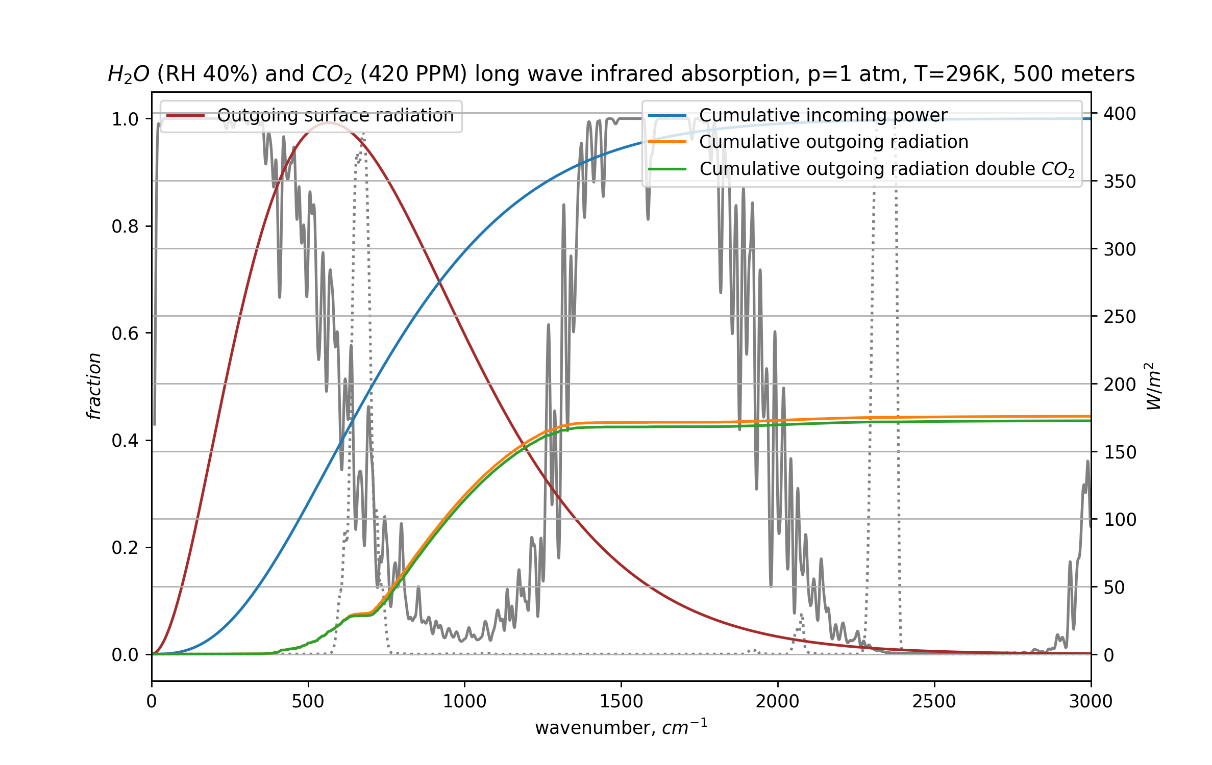
This is a graph of the same atmosphere, with superimposed the infrared radiation coming from the ground (in brown). This radiation gets absorbed by the CO₂ and H₂O in the 500 meter of atmosphere we are modeling here. On the right axis, the cumulative radiative power over all frequencies is plotted. So, the total power coming from the surface (in blue) is a shade under 400W/m2.
The orange line denotes the cumulative radiative power after absorption by 500 meters of atmosphere, the part that continues upwards, and this is just 163W/m2. The green line below that is the most interesting part of this graph: how much infrared radiation gets out when we double the CO₂ concentration. And this is around 5W/m2 less.
With this we’ve already refuted a main claim of the “CO₂ is saturated theory” – more CO₂ definitely makes it harder for the Earth to radiate heat away into space, even in this most saturated part of the atmosphere. In the first 500 meters, this mostly happens because the range of frequencies where CO₂ blocks radiation best (around 700cm-1) actually gets wider as the concentration doubles. So the blocking is not necessarily more powerful locally, just more of it happens. More about this later.
Here we’ve reached a key point of how even pre-industrial level greenhouse gases work to keep the Earth at its “normal” temperature. The lower atmosphere indeed blocks most outgoing radiation. But what happens if we go higher up the atmosphere?
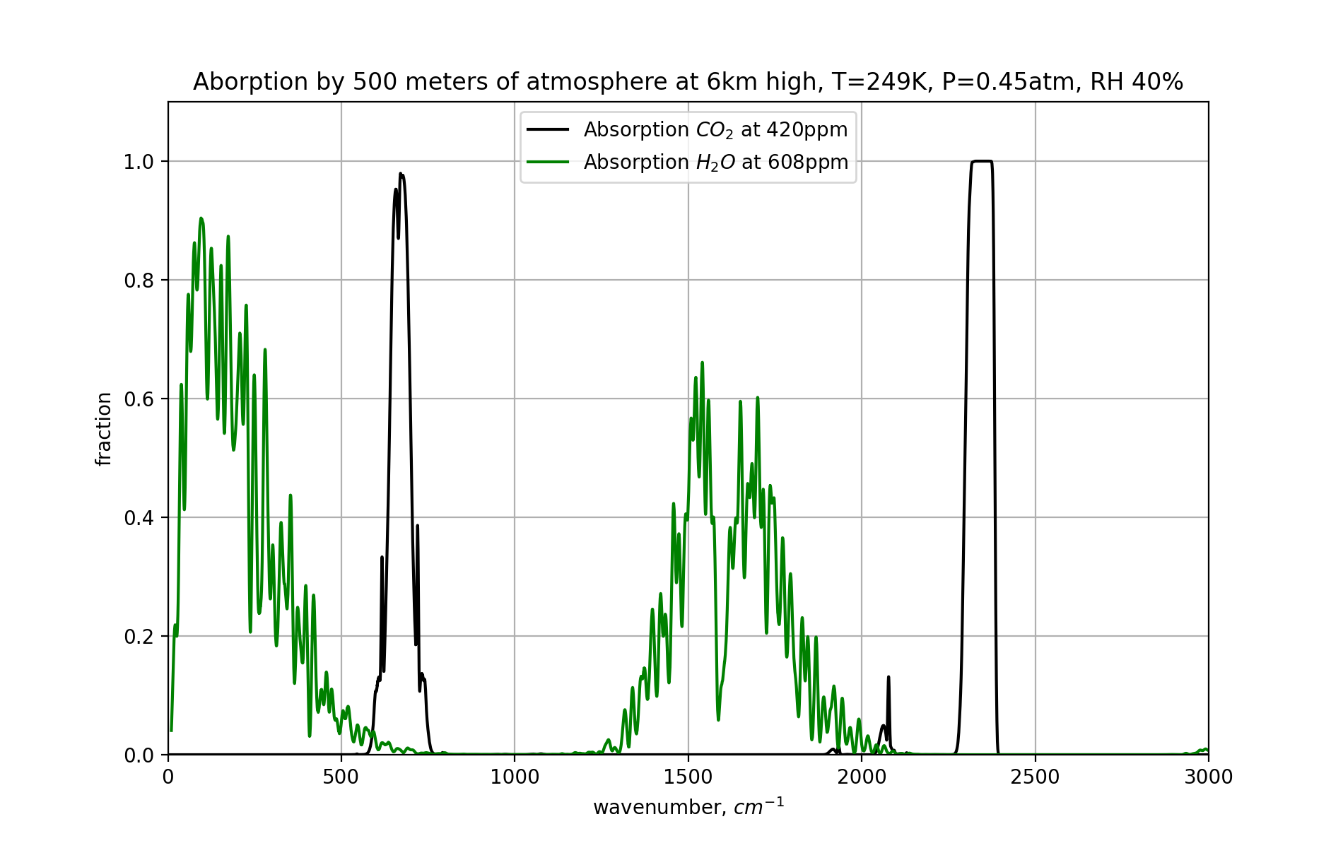
At 6 kilometers, the amount of CO₂ molecules has gone down, simply because the ambient pressure is lower. The concentration is still 420 ppm but those million particles are a lot more spread out now. For water, the effect is much more dramatic - at , air can not hold a lot of water, and we’ve gone from 10,000 ppm to only 608 ppm.
From the graph we can see that the water frequencies are ‘opening up’ at 6km high, and most light of those wavelengths can escape to space. The CO₂ band however remains pretty closed, so not all frequencies of light can get out. But a lot can.
Recall how earlier we established that the radiating part of the earth needs to be around , but that this does not necessarily need to come from the actual surface. And it doesn’t, since the lower atmosphere provides great insulation. However, here at 6km high we see that outgoing radiation is possible. And thus we’ve (more or less) found the range of the atmosphere where radiation happens. And this zone then needs to be around , to get the power of the outgoing radiation right.
Earlier this post described the lapse rate on Venus, where the atmosphere gets hotter as you descend to the surface. On Earth the same thing happens, and the environmental (effective) lapse rate is around 6K per kilometer, which means that in order to have an atmosphere of at 6 kilometers high, the surface needs to have a temperature of + 6 * = . The reality is around (on average), so this is a pretty good result.
Now, as previously, this number is pretty good mostly because we got lucky. This is a spherical cow kind of calculation. But it is still encouraging that we get mostly the right number.
The specific oversimplification here is that the spectrum to outer space opens up at different elevations for different frequencies of light. In reality there is not one ’emission zone’. Also, once water is gone from the atmosphere, the outgoing radiation is no longer a simple black body affair. Gas can only glow in frequencies which it absorbs. However, at 6km high with the water vapor still in there, the simple black body approach still works well enough for this spherical cow.
So what happens if the CO₂ concentration increases?
The water part of the spectrum opens up at around 6 kilometers in our simple model. If for some reason there were more water in the atmosphere, we might have to go up higher before radiation to space picks up. And due to the lapse rate, this would (over time) lead to a higher surface temperature.
We could get confused by this - it is not that the lapse rate heats the surface. It is that the surface needs to be a certain temperature so that, taking into account the lapse rate, the radiating part of the atmosphere ends up at . If the surface starts colder than required to do so, the radiated power into space will be less than what is coming in (because the radiating part is perhaps). This means there is excess energy, which will eventually make the surface hot enough so that equilibrium is reached. Confusion on this subject has tripped up many luminaries.
This rising process is often incorrectly wheeled out to explain how more CO₂ leads to more global warming (which it does), but CO₂ is different than water vapor in this sense. As noted above, the whole atmosphere does not open up in unison once you get high enough:

I must stress that this is a rough sketch meant to illustrate a point - don’t take the numbers too seriously
Here we see that the water parts of the spectrum indeed do open up at 6km (in our model), but that for CO₂ this only happens at 20 kilometers high or more. It may also be interesting to note the window around 1000 cm-1, which radiates out into space straight from the surface. With clever materials, this window can be used for passive cooling.
Of additional note is the dashed line representing the stratosphere. We’ve previously described how the lapse rate causes a temperature differential of /km, but this rule only holds for a well mixed atmosphere. And at a certain height, the atmosphere stops being mixed like that. Once we hit the stratosphere (somewhere between 9 and 20km up), the temperature no longer decreases, and in fact, after a while starts to go up again.
When the CO₂ concentration goes up, this will indeed also raise the height in the atmosphere where the CO₂-absorbing part becomes transparent. However, since the temperature profile is flat in that part of the stratosphere (20km), this will not have any lapse rate effects that impact the surface temperature. Unlike water, for which this ceiling is well below the stratosphere.
There is another effect however:
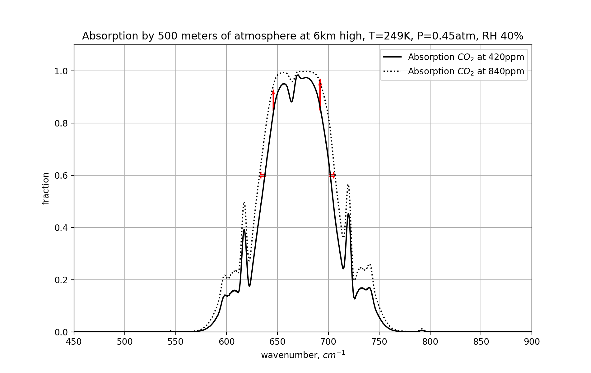
This is a close-up of the absorption graph for CO₂ in the 550-800 wavenumber range. The left and right “wings” of the part of the spectrum blocked by CO₂ expand with a higher CO₂ concentration. Frequencies that were previously not meaningfully absorbed now do get absorbed significantly. And wavelenghts that were already absorbed, but only to a certain elevation in the atmosphere, now get absorbed until greater heights. And this causes the lapse rate to have a bigger effect again (for these wings).
Now, seen from this graph, the effect of even a doubling of CO₂ doesn’t appear to be too big, maybe a few percent. But a few percent of 400W/m2 of heat radiation is sufficient to cause whole degrees of warming. But, there’s more.
So, how much will a doubling of CO₂ warm the planet?
Our spherical cow model has a few parameterized items in there. These are numbers that we don’t calculate or simulate, but copy from a table somewhere. “Non-playable characters” as it were. These include the albedo of the Earth (30%), the temperature of various layers of the atmosphere, but also the assumed water content of the atmosphere. To fully predict what will happen, we need to let these parameters evolve. Of specific note is the water content. The warmer air gets, the more water it can contain, even at steady relative humidity (which we assumed to be 40%):

The Clausius-Clapeyron relation means roughly 7% more water mass for every 1K increase in temperature
A CO₂-caused increase of temperature in turn attracts more water molecules to the atmosphere, which trap more radiation, thus amplifying the original warming. This effect doesn’t go on indefinitely of course, but the amplification makes CO₂ even more important.
Here is what that means for the height at which the atmosphere starts to radiate:

Doubling CO₂ (1) slightly impacts the absorption by CO₂ itself, and (2) the subsequent warming increases the amount of water vapor in the atmosphere, and that in turn raises the elevation at which the H₂O bands become transparent
In this way more CO₂ means more water vapor, which means the water vapor bands in the atmosphere only open up at a higher altitude. And that means more the lapse rate works on a larger vertical range, which in turn requires a hotter surface so the radiating layer is hot enough to radiate enough heat into space.
If you run the numbers (including water) using relatively simple models, as Gilbert Plass did in 1955, Manabe and Wetherald in 1967 or Svante Arrhenius in 1896, you find that doubling the CO₂ concentration results in a perhaps 2-4 degree warming of the surface.
More sophisticated general circulation models take into account ocean flows, rain, snow, ice, cloud formation, more greenhouse gases, aerosols and many other factors. These models sadly come to quite a range of conclusions, but all of them predict multiple degrees of warming per CO₂ doubling.
Crucially, it is incredibly hard to think of a mechanism where CO₂ would not drive heating.
If water is so important, why fret about CO₂
Water is in a way the most important greenhouse gas there is. The reason we obsess over CO₂ is that we are emitting vast quantities of it, and we could stop doing that. Meanwhile, the relative humidity of the Earth is stubbornly stuck somewhere around 40%. It is not something we can drive, it happens because water just happens to work like that at certain temperatures and pressures. The concentration of water vapor is indeed going up slightly, but this is what happens with rising temperature.
And 30% albedo?
The Earth reflects 30% of light straight back into space. If you could change that to even 31% all our global warming would be gone. And unlike water, it appears we do have a hand in this albedo. Reflection happens by clouds, which we don’t understand well enough, but also by aerosols. Aerosols include (desert) dust, soot and other man-made materials. Some aerosols live very high up in the atmosphere, where they have effects on sunlight without polluting the ground level air. I wrote about this earlier.
All climate calculations hinge crucially on this albedo percentage, and even in our spherical cow model the albedo has a huge influence on temperature. There are indications the albedo is going down a bit leading the Earth to absorb more solar radiation, possibly because we are polluting less.
Although changing the albedo could really matter, eventually it would lose out against ever increasing amounts of CO₂. So even if we could do it, modifying the albedo on its own would not really save us in the long run.
Methane, other greenhouse gases
These certainly don’t make things any simpler. To keep the already complicated graphs on this page comprehensible I’ve left out methane, ozone and N2O. That is not because these gases are not important, but because these molecules do not hang around for a long time in the atmosphere. Every gram of CO₂ we emit will continue to heat us up for centuries.
Adding the other gases to the graphs and calculations above does not change their results materially - because the model used is so simple.
Nevertheless, in real models, it is very clear that reducing methane emissions would be very helpful in the short run.
Atmospheric radiative transfer models
In reality, things are more complicated. For example, we’ve been picking the pressure and temperature for the atmosphere at different heights from the international standard atmosphere table. In doing so we’ve parameterized part of our model, where we don’t calculate/model some values but simply pick them from a table.
Real models take into account what happens to the absorbed radiation. Not only the solid Earth radiates blackbody (Planck) radiation, so do opaque parts of the atmosphere. So our 500 meter thick slice of the atmosphere actually radiates energy up and down again, based on its temperature, influencing temperatures in the rest of the atmosphere.
To model this process, atmospheric radiative transfer models are used, and these are very complex, but can predict the spectrum of outgoing longwave radiation very well.
In such models, the transfer of photons from the surface into space is simulated or calculated, and the end result shows how much energy is leaving the earth, and at what frequencies. There is very good correspondence between what the models produce, and what is being measured from space.
Simultaneously, it is quite shocking to read on the ESA website that “the far-infrared part of the [outgoing] electromagnetic spectrum has never been measured from space before.” ESA is launching a satellite to fix this already in 2027.
Oddly enough it seems we are measuring the atmosphere of Mars better than our own atmosphere.
Summarising
Our simple model allowed us to calculate a plausible temperature for the Earth’s surface. Initially 30% of sunlight gets deflected back to space. If the Earth were an unshielded black body radiator, this would lead to an average surface temperature of . However, the surface is in fact shielded, mostly by water vapor and CO₂. This means the surface can be hotter. As we go up in the atmosphere, the warming shield becomes ever thinner, and heat starts to escape into space. In our simple model, this starts to happen at around 6km of elevation. There the air must then be (on average), the temperature we calculated earlier for a perfect black body Earth.
If the air is at 6km high, the ground must by 6*= degrees warmer to make that happen, because of the lapse rate. This gives us a ground temperature of , close to the actual average of .
This is a very simple model of how even pre-industrial greenhouse gases keep us warm.
The (saturated) absorption bands of CO₂ and water vapor are indeed able to trap almost all thermal emissions from the surface within their respective frequency ranges. Doubling the CO₂ concentration broadens the CO₂ bands slightly, and that is how more CO₂ effectively leads to more warming: the saturated parts don’t trap yet more infrared light, but there are more frequencies where CO₂ is saturated at a doubled concentration. So net, there is more absorption.
This further insulation causes a temperature rise, which in turn causes more water vapor to enter the atmosphere. Water vapor in itself is also good enough at trapping infrared radiation that at lower elevations, it’s effect is also saturated. However, this is no longer the case higher up, since colder air contains a lot less water. The CO₂ caused warming increases the absolute humidity (concentration) of water, causing it to continue to block outgoing radiation until higher levels of the atmosphere.
And because this raises the ceiling of where outgoing radiation into space happens, again the lapse rate means that the Earth’s surface must heat up to maintain the temperature at the new radiating level.
In this way, an increase in CO₂ concentration itself causes warming, and water vapor further amplifies that.
Simple models do not allow us to predict with great certainty just how much warming this will be, but all models predict warming, and many of them tell us there will be over 3C/5F of warming in case the CO₂ concentration doubles.
Next up & concluding
If this page has failed somewhere in explaining things (and this is entirely possible), it might be that viewing dr Sabine Hossenfelder’s video could plug the gap.
The video and this page necessarily have to leave out a lot of detail. But once you truly get this “spherical cow” model, you can far more easily delve into the things that we’ve not talked about, like the role of other greenhouse gases, or collision induced absorbance (‘CIA’), or the interaction between UV radiation and ozone in the stratosphere, stratospheric water vapor and many other exciting fields of study.
It is also important to know that there is more to global warming than just atmospheric gases. Clouds are a major open question for example, and we don’t understand them well. Biology might also play a larger role. Our environmental pollution might paradoxically have been keeping us cooler. Our little model can’t encompass this all.
However, what you will now in any case be able to do is rebut people who claim CO₂ is saturated and that more CO₂ will therefore not be a problem. You can point doubters at this page, which they might not read, but at least you have something to point at.
If you have any questions or suggestions for this page, please do contact me on bert@hubertnet.nl
And before you send me a paper to look at, please run it through the checklist in the companion blog post with more details to see if it is a useful article.
Thank you for making it to the end of this page!
Extra thanks
Maciej Chmielarz provided very helpful feedback on readability and also spotted many mistakes.
Two anonymous climate scientists from a major institute kindly suggested additional papers, which helped this article to become more factual.
I’m also indebted to Eli Mlawer for providing reassurance on the proper use of the key Mlawer-Tobin-Clough-Kneizys-Davies water vapor continuum spectrum model.
This page also makes extensive and grateful use of the HITRAN molecular absorption database, another mainstay of atmospheric climate research.
Further reading/viewing
- The companion blog post with more code and physics
- HITRAN, the high-resolution transmission molecular absorption database. HITRAN is a compilation of spectroscopic parameters that a variety of computer codes use to predict and simulate the transmission and emission of light in the atmosphere.
- European sort of equivalent project: GEISA, GEISA 2020.
- LibreTexts Introduction to Infrared Spectroscopy , by Thomas Wenzel
- The influence of the 15 u carbon-dioxide band on the atmospheric infra-red cooling rate by Gilbert Plass
- ARTS: The Atmospheric Radiative Transfer Simulator
- Thermal Equilibrium of the Atmosphere with a Given Distribution of Relative Humidity , Nobel prize winning paper setting out how global warming works
- 2019 Followup: Role of greenhouse gas in climate change. Useful because it goes beyond just atmospheric transfer models. This paper describes the same radiative transfer modes as in this blog post, but uses different language, a different way to look at it. This might work better for you (or worse), but is in any case stimulating. It is the same model though.
- Global Warming - The Complete Briefing - comprehensive and accessible book. Takes a broad view. Here’s an apparently free PDF of the third edition from 2004.
- Principles of Planetary Climate. Big serious academic book. Paints a full pictures in great detail. Lots of math.
- Ice melt paper
- Global warming in the pipeline, preprint by James E. Hansen et al.
- RMetS paper explaining basics of CO₂ saturation
- Saturated gas rebuttal on real climate
- Infrared radiation and planetary temperature
- Wikipedia on atmospheric methane: Methane is a major source of water vapour in the stratosphere through oxidation and water vapour adds about 15% to methane’s radiative forcing effect
- Graphs of H₂O absorption with/without continuum
- Using earthshine to measure Earth’s albedo
- 1977 paper with the origin of the “radiation field”
- Article with details on size of continuum spectrum: The continuum amplitude is small compared to the absorption at the center of resonance lines. Nevertheless, its integrated contribution to the atmospheric absorption is larger than the contributions from major greenhouse gases as CO₂ and CH4.
- On current climate models running too hot
- Great collection of “warming papers”
- The higher frequency continuum spectrum
- Shine, K. P., Ptashnik, I. V., & Rädel, G. (2012). The Water Vapour Continuum: Brief History and Recent Developments. Surveys in Geophysics, 33(3-4), 535–555.
- The water vapor self-continuum in the “terahertz gap” region (15–700 cm–1): Experiment versus MT_CKD-3.5 model
- Hossenfelder video
- sixty symbols video of saturated CO₂
- Climate sensitivity, state dependence
- Line by line radiation transfer model
- Earth’s outgoing longwave radiation linear due to H₂O greenhouse effect alternate link
- International Standard Atmosphere